An Introduction to Triangled Equilateral Triangles
“I've been a long time coming, and I'll be a long time gone. You've got your whole life to do something, and that's not very long.”(Ani DiFranco)
One of the generalisations discussed by Brooks, Smith, Stone and Tutte in "The Dissection of Rectangles into Squares" (1940)[1] was the dissection of triangles into triangles. Some forty years later Tutte wrote ; "I have no cause to complain about the reception of papers on squared rectangles by mathematicians and other scientists. They are all pleased that there should be a connection between Kirchhoff's Laws of electrical flow and the dissection problems of pure geometry. But there seems to be no corresponding interest in the triangular problem. Yet in my opinion the theory of triangulated triangles is a simple and elegant generalisation of those theories of squared rectangles. ... "[2].
At about same the time Tutte wrote those words, A student of Duijvestijn, Lex Augusteijn was working on his bachelors thesis[25] at Technische Hogeschool Twente. The thesis was completed in June 1980, it was called Triangulations and this is a quote from the introduction;
The problem of the dissection of parallellograms and triangles into equilateral triangles has got less attention than the dissection of rectangles into unequal squares. On the squaring problem many papers have been written to find the lowest order simple perfect squared square (found in 1978 by Duijvestijn). However, the problem of triangulation seems to be studied only by Tutte. His work (and especially the representation by digraphs and his "electrical model") has been very helpful to us in undertaking the computer search for the lowest order triangulated parallellogram, cylinder, triangle and rhombus, here described.The results of Augusteijn's search are summarised in the following table (taken from page 25 of his thesis[25])'
| Order | Parallelogram | Cylinder | Triangle | Rhombus |
|---|---|---|---|---|
| 6 1/2 | 20 x 19 | 21 x 20 | - | - |
| 7 | - | 28 x 29 28 x 23 |
- | - |
| 7 1/2 | - | 36 x 38 33 x 35 39 x 32 37 x 41 37 x 41 36 x 35 35 x 40 36 x 29 |
39(c) | - |
| 8 | 48 x 42 47 x 43 47 x 44 |
17 cylinders | 48(c) | - |
| 8 1/2 | 16 ones | not calculated | all compound | - |
| 9 | many | not calculated | 45 90 48 48 91 many compounds |
- |
It took another thirty years before another attempt was made to enumerate triangulations. In July, 2010 Aleš Drápal and Carlo Hämäläinen published : An enumeration of equilateral triangle dissections. (Discrete Applied Mathematics, Volume 158 Issue 14). We provide a brief explanation of their work and display below some of their catalogue of equilateral triangle dissections, but to understand what they, and Lex Augusteijn have done, we need to provide a rather detailed introduction to the subject of equilateral triangle dissections and associated topics. In so doing we make use of expository articles by W.T. Tutte and Augusteijn, see the references at the end for even more detailed technical information. The selection of quotes for headings is due solely to Stuart Anderson.
'There and back again.'(J.R.R. Tolkien)

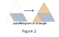
"When we are discussing dissections into equilateral triangles it does not really matter whether the original figure is a triangle or a parallelogram (with angles of 60° and 120°). A dissection of a triangle can be changed into that of a parallelogram by deleting one constituent triangle (at a vertex) and adding another. A dissection of a parallelogram can be changed into that of a triangle by adding new constituent triangles on two adjacent sides."[2]
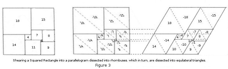
"It is the dissected parallelogram that is the natural analogue of the squared rectangle. Suppose we start with a squared rectangle R and shear it so that it becomes a dissection of a parallelogram into rhombuses. Each rhombus can be dissected along an appropriate diagonal to form two congruent equilateral triangles. The squared rectangle R is thus transformed into a triangulated parallelogram P. Because of this observation we can regard the theory of squared rectangles as a special case of the theory of triangulated parallelograms."[2]
"A beautiful thing is never perfect.”(anon)
Suppose that R is a perfect rectangle. Does it make sense to say that P is perfect also? Strictly speaking no, Tutte explains[7], "I remember Stone demonstrating , at a meeting of the Four, that in any dissection of an equilateral triangle into smaller ones there must be two constituent triangles with the same (absolute) side length. The same is true for dissections of parallelograms. Perhaps we should say that a dissected parallelogram can be perfect, but not absolutely perfect. Stone got his result by applying the Euler Polyhedron Formula to the "electrical network" of a triangulated triangle." David Radcliffe provides the proof here.. However all is not lost, one can recover a notion of 'perfection' by treating triangles pointing up and triangles pointing down as different, Tutte explains [2]; "Given any triangulated triangle or parallelogram we can fix one of its sides as "horizontal". Then any constituent triangle T has one horizontal side. Let us say that T is positively or negatively oriented according to its position above or below its horizontal side. Let us define the "size" of T as plus or minus the length of its side, depending on whether T is positively or negatively oriented. Then we say that a triangulation is "perfect" if no two of its consituent triangle have the same size. With this definition we can say that the perfect rectangle R shears into a perfect parallelogram P. For the two congruent triangles of P, arising from any square of R, have opposite orientations and therefore have different sizes."
“Call it a clan, call it a network, call it a tribe, call it a family: Whatever you call it, whoever you are, you need one" (Jane Howard)
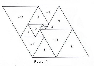
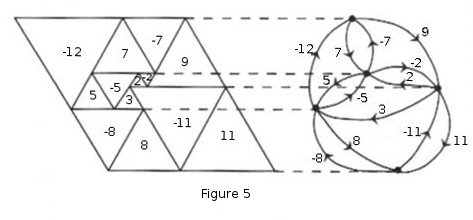
"Figure 4 shows a perfect parallelogram that cannot be obtained by shearing a perfect rectangle. In [6] I have satisfied myself that this parallelogram has the least number of constituent triangles, namely 13, consistent with perfection. For the sake of comparisons with squared rectangles, I like to say that its order is 13/2. For each square of a rectangle corresponds when sheared to two triangles. The number entered in each triangle of Figure 1 is its size."[2] At this stage in papers on squared rectangles, there appears a diagram showing the relation between a squared rectangle and its electrical network. Figure 5 fulfills the same purpose in the theory of triangulated parallelograms. But now the term "electrical" must be used in a generalised sense. It refers to a form of electricity not yet found in physics. Each horizontal segment in a triangulated parallelogram is represented by a vertex of the electrical network, just as in the case of a squared rectangle. Each triangle is enclosed between two horizontal segments, its base being in one and its apex in the other. It is represented in the network by an edge joining the two corresponding vertices. But this time it is a directed edge, a dart, the arrow going from apex to base. Against each directed edge is written the side length of the corresponding triangle, positive or negative, we call this is the current. We say that the upper and lower sides of the parallelogram correspond to the positive and negative poles of the network respectively.
There is a natural anticlockwise cyclic order of the triangles meeting a given horizontal segment by base or apex. We exclude triangles meeting the segment in any other way, of which there are at most two, one at each end. In this cyclic order triangles meeting by base alternate with those meeting by apex. We contrive to preserve this cyclic order in the directed graph. Then at each vertex of the network, incoming edges alternate with outgoing ones. All this is done without edge-crossings, and so our diagram determines a planar map. Let us call it an "alternating map" to emphasize the alternation of incoming and outgoing edges at each vertex. Let us also record the obvious fact that the number of edges at each vertex is even.
"Electricity is of two kinds, positive and negative. The difference is, I presume, that one kind comes a little more expensive, but is more durable; the other is a cheaper thing, but the moths get into it." (Stephen Leacock)
If we look at the horizontal lines in the dissected parallelogram of Figure 4 or Figure 5, the length of each horizontal line is equal to the length of all the triangle bases that meet it on the upper side and also equal to the length of triangle sides that meet it on the lower side. Translating this to the accompanying network N, the "alternating map", the currents incoming to a vertex v are called the current leaving N at v.. Its negative is the current entering N at v. Thus, the current entering the positive pole is equal to the current leaving the negative pole, and each of these numbers measure the length of a horizontal side of P. But the current entering or leaving N at any non-polar vertex is zero, and the current leaving is the sum of the sizes of the triangles of P having their bases in the corresponding horizontal segment. This rule of currents at non-polar vertices is our analogue of Kirchhoff's First Law. However the zero sum is not over all incident edges but only over the incoming ones. Kirchhoff's Second Law persists unaltered. We assign to each vertex a "potential" equal to its distance, measured at a slant of 60° above the base of the parallelogram. then the current in an edge is the potential at the tail of its arrow minus the potential at the head. It follows that the total change of potential around any circuit is zero, as required by Second Law.
"Recipes are like poems; they keep what kept us. And good cooks are like poets; they know how to count."(Henri Coulette)
We are now at the point where we can write down an algorithm - a 'recipe' or procedure for constructing an equilateral triangulated triangle. Essentially what we do is reverse the steps above. ie
- Draw an alternating map.
- Choose positive and negative poles on the boundary of the outer face of the alternating map.
- Calculate the currents in the wires by solving the modified Kirchhoff equations for both arrow directions.
- Reverse the construction of Figure 5 to create a parallelogram from the alternating map currents.
- Add two extra triangles to create an equilateral triangulated triangle from the parallelogram.
"There is a theory which states that if ever anyone discovers exactly what the Universe is for and why it is here, it will instantly disappear and be replaced by something even more bizarre and inexplicable. There is another theory which states that this has already happened." (Douglas Adams)
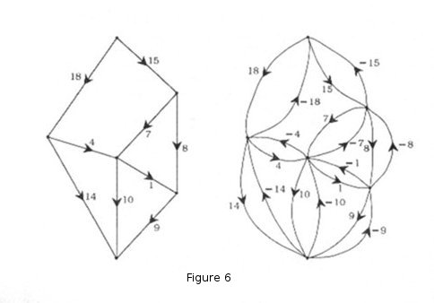
What is the theoretical justification for our 'recipe'? we can say that the theory of triangled triangles is closely related to the theory of squared rectangles, indeed it is a generalisation of that theory. To see this we go back to the diagram of the sheared squared rectangle changing into the parallelogram. Now in Figure 6 we show the graphs that are associated with the squared rectangle and the parallelogram. We see on the left the ordinary electrical network of the 33x32 squared rectangle, and on the right we see the new-style electrical network of one of its shear-derived triangulated parallelograms.
The main change in going from left to right is that each wire is doubled; it is replaced by two oppositely directed edges. The ordinary Kirchhoff equations for the first network are identical with the modified ones for the second. So the device of doubling edges exhibits the theory of squared rectangles as a subcase of the theory of triangulated parallelograms.
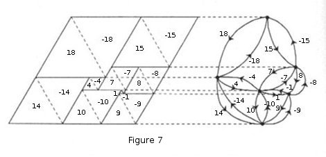
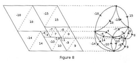
The doubling and directing must be done so as to give an alternating map. Actually this can be done in two ways, corresponding to the left and right shearings of the rectangle. As an example we can take the new-style electrical networks appearing in Figures 7 & 8. The change from the first diagram to the second is simply that the direction of each edge is reversed. It is as a consequence of this reversal that each current is multiplied by -1. More generally we can observe that the reversal of all edges changes one alternating map into another.
The theory of squared rectangles is itself based on electrical network theory, worked out in the 19th century by Kirchhoff and Maxwell. Kirchhoff stated the basic formulas for mesh equations in 1847 and Maxwell gave the basic formulas for the node equations in 1872. A network, in the context of electronics, is a collection of interconnected components. Network analysis is the process of finding the voltages across, and the currents through, every component in the network. There are a number of different techniques for achieving this. However, for the most part, they assume that the components of the network are all linear. Kirchhoff encoded the graph G of the network N into a matrix called the Kirchhoff or Laplacian matrix, denoted K(N) by Tutte et al. which is the difference between the graph's Degree matrix (a diagonal matrix with vertex degrees on the diagonals) and its Adjacency matrix (a (0,1)-matrix with 1's at places corresponding to entries where the vertices are adjacent and 0's otherwise). The Laplacian matrix can also be obtained by multiplying the Incidence matrix of G by its transpose.
I did not look for matrix theory. It somehow looked for me." (Olga Taussky Todd)
The Matrix-Tree Theorem states that the number of spanning trees is equal to the absolute value of any cofactor of the Laplacian matrix of G. For a general electrical network N it is equal to the sum over all spanning trees of N of the products of the conductances of their edges. Some necessary graph-theoretical background is required. Let G be a finite graph. We say that G is connected if there exists a walk between any two vertices of G. A cycle is a closed walk with no repeated vertices or edges, except for the the first and last vertex. A tree is a connected graph with no cycles. In particular, a tree cannot have multiple edges, since a double edge is equivalent to a cycle of length two. A spanning subgraph of a graph G is a graph H with the same vertex set as G, and such that every edge of H is an edge of G. A spanning subgraph which is a tree is called a spanning tree. G has a spanning tree if and only if it is connected. The number of spanning trees of a graph G, is sometimes called the complexity of G and often denoted K(G).
By definition the Laplacian matrix is symmetrical and the elements in each row and column sum to zero, thus det K(N) = 0. The determinant of the matrix Ki(N) obtained from K(N) by striking out the ith row and column is independent of i. We call this a cofactor of K(N). Its value is the complexity C(N) of N. it is positive for all connected N and zero for disconnected networks. If C(N) is taken as a measure of the total current entering at the positive pole and leaving at the negative pole, then the potential drop, the voltage between the two poles was, according to Kirchhoff and Maxwells theory, the determinant of the matrix obtained from K(N) by striking out the rows and columns of the two poles, we call the full potential drop from v1 to vn to be K1n(G), where K1n(G) is the matrix derived from K(G) by striking out the first and last rows and columns. Other determinants derived from K(N) give the potential drops between specified pairs of vertices, and thus the currents in the individual wires. From this it can be inferred that if the horizontal side of a squared rectangle is made equal to the complexity of the corresponding electrical network, then both the sides of the rectangle and the sides of all the component squares are integers. In some cases it was possible to divide all these integers (the full sides and full elements) by a common factor called the reduction factor, this leaves us with what we call the reduced sides and the reduced elements, all now having a GCD of 1.
"It's the little details that are vital. Little things make big things happen." (John Wooden)
When applying the Matrix-Tree theorem to the alternating maps of triangled parallelograms the Laplacian matrix is defined slightly differently. The jth diagonal entry cjjis the number of darts coming to vertex vj from other vertices. The non-diagonal entry cjj in the ith row and jth column is minus the number of darts directed from vj to vi. The elements of K(G) sum to zero in the rows but not in every column, but this is still enough to ensure det K(G) = 0. As before we define the complexity Ci(G) of G at vi as det Ki(G), where Ki(G) is the matrix obtained from K(G) by striking out the ith row and column. In the case of alternating maps the elements of K(G) sum to zero in both rows and columns so the determinant is independent of i (the ith row and column is struck out), so the complexity is the same at every vertex. For squared rectangles The Matrix-Tree theorem applies to an undirected graph. In this case the Matrix-Tree theorem is generalised to apply to directed graphs. It says that Ci(G) is the number of spanning trees diverging from vi, meaning each edge is directed away from vi in the tree.
We can express the equations in matrix form. If we rename Ki(N) as A, and a vector of node voltages as x, we can write Ax=b, b=0 where x is the nullspace of A and the equation expresses Kirchhoffs first law. To solve it we multiply both sides by the inverse of A. A*Inverse(A) cancels out, giving x = Inverse(A)*b. If we invert A we can find x, the node voltages. In practice we use LU decomposition to factor the matrix into its lower triangular and upper triangular factor matrices. This can be done efficiently on a computer. Once we have the node voltages, the currents can be obtained as the differences of the voltages at each edge. This can be easily done with matrices also.
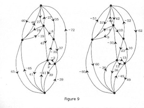
We return to the operation of reversing every dart in a network. For an alternating map, it replaces K(G) by its transpose. It then likewise replaces K1(G) and K1n(G) by their transposes, and so does not alter their determinants. Hence if G is the graph of an alternating map the operation alters neither the horizontal side nor the slanting side of a corresponding triangulated parallelogram. Nevertheless it may change the set of full currents in the wires of the network, and therefore it may alter the set of constituent triangles in the parallelogram. It may even happen that the two triangulations have no triangle in common apart from the overall triangle. Figure 9 gives an example of two alternating maps identical except for a reversal of the darts, the networks are shown (but not the parallelograms).
How do alternating maps relate to the two graphs of squared rectangles, which are duals of each other? To answer we go from triangulated parallelograms to triangulated triangles. In Figure 2 we showed how a parallelogram can be changed into a triangle by adding two triangles to adjacent sides of the parallelogram.
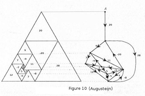
In Figure 10 we start with a triangulated parallelogram, add 2 triangles and draw its network. The network shows the horizontal segments as vertices and the triangles as directed edges - darts, just as for a parallelogram, except that there is an extra vertex A to represent the apex of the triangle. This extra vertex is the positive pole of the network. The electrical network is not that of an alternating map, but this defect is easily corrected by identifying the two poles. Let us note that the current entering the network at the positive pole is zero. This is in accordance with the Matrix-Tree theorem, since there can be no spanning tree diverging from any vertex other than the postive pole, and therefore the complexity at the negative pole is zero.
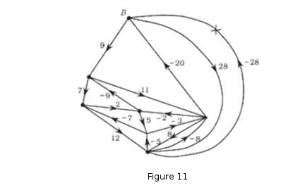
Figure 11 shows the electrical network obtained from that of Figure 10 by identiying the 2 poles. The edge incident with the positive pole A in Figure 10 we call the "polar edge" of the new diagram and mark it with a cross. If we assign it a current -28 we get the electrical network of a parallelogram, complete with currents. That parallelogram is obtained from the triangled triangle by suppressing the constituent of size 20 and adding a new one of size -28 on the right. It can be shown that the complexity of the new network is equal to that of the original at A.
A triangled triangle can be oriented in 3 different ways (rotation by 0°, 60° and 120°). Generally in each case the horizonal lines are different and the three network graphs produced are different. These three network graphs can become three different alternating maps when poles are identified. This procedure is analogous to the construction of two dual c-nets from the two sets of parallel segments in a squared rectangle. How do the three alternating maps relate to each other? They are not duals. Tutte called them 'trine' -(a term borrowed from astrology, possibly the only useful thing to come from astrology into science in modern times), The property they exhibit is not 'duality' but triality, later called 'trinity'.
Brooks, Smith, Stone and Tutte worked on how to best fit the three trine maps together into one diagram, and C.A.B. Smith came up with the answer. Smith showed that the three trine maps can be constructed from a single planar bicubic map. A "bicubic" map is a graph drawn in the plane that is both cubic and bipartite. In a cubic map every vertex has exactly three edges incident. With a bipartite map, each vertex can be coloured black or white (or + or -) so that a black vertex has only white neighbours and vice versa. P. J. Heawood showed that a bicubic map can be face coloured in three colours if and only if it is bicubic.
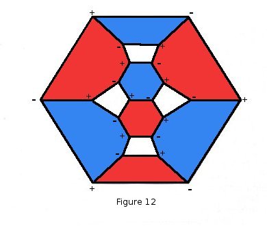
We can derive an alternating map from a bicubic map (Figure 12) as follows; The faces coloured red are designated as alternating map vertices. The black edges separating the white and blue coloured faces are the alternating map edges. Each of these is directed from its negative end to its positive, making the darts of the alternating map. Finally we shrink the red faces down to vertex points and we have an alternating map. We can repeat the process starting with a blue or white colour, giving us the three alternating maps of the triangled triangle. We can also run the process in reverse, creating a bicubic map from alternating maps.
Tutte was able to prove that the three trine alternating maps have equal complexities, just as do two dual c-nets.
With bicubic maps, we can extend the above 'recipe'. If we have a supply of bicubic maps, we should be able to make alternating maps, and from them, triangulated triangles.
One needs a graph generator to produce the bicubic maps. The generator should produce all possible maps in the given class, but not produce duplicates, so we need a fast, efficient non-isomorphic exhaustive map generator. The map generator should be able to produce maps according to a specified number of vertices and edges, this would enable us to produce, and count, all dissections of an equilateral triangulated triangle with a certain number of triangles in the same way that we produce all squared rectangles with a given number of squares (the order). It would also be preferable if the generator produced verifiable and proven results in accordance with established graph theory and if the source code was freely available to researchers, mathematicians, computer scientists, students, and triangle dissectors. Fortunately such a generator exists, its name is plantri, it has been created by Brendan McKay and Gunnar Brinkmann and is available from Brendan McKay's website. If we check the plantri manual we find plantri can produce bicubic maps by running the program with the -b and -d switches.
How does the above method, described by W. T. Tutte compare to the method of Aleš Drápal and Carlo Hämäläinen?
“Our similarities are different.” (Philip James Bailey)
The method of Aleš Drápal and Carlo Hämäläinen uses latin bitrades to dissect equilateral triangles. Cavenagh and Lisoněk[8] showed that spherical latin bitrades are equivalent to planar Eulerian triangulations. Planar Eulerian triangulations are the duals of bicubic maps. To enumerate triangle dissections Drápal and Hämäläinen also use plantri. Quoting from their paper [3];
"Consider an
equilateral triangle ∑ that is dissected into a finite number of equilateral
triangles. Dissections will be always assumed to be nontrivial so the number
of dissecting triangles is at least four. Denote by a, b and c the lines induced
by the sides of ∑. Each side of a dissecting triangle has to be parallel to one
of a, b, or c. If X is a vertex of a dissecting triangle, then X is a vertex of
exactly one, three or six dissecting triangles. Suppose that there is no vertex with six triangles and consider triples (u; v; w) of lines that are parallel to a,
b and c, respectively, and meet in a vertex of a dissecting triangle that is not
a vertex of ∑. The set of all these triples together with the triple (a; b; c) will
be denoted by T*, and by T∆ we shall denote the set of all triples (u; v; w)
of lines that are yielded by sides of a dissecting triangle (where u, v and w
are again parallel to a, b and c, respectively). The following conditions hold:
(R1) Sets T*, and T∆ are disjoint;
(R2) for all (p1; p2; p3) ∈ T* and all r, s ∈ { 1; 2; 3} , r ≠ s, there exists exactly
one (q1; q2; q3) ∈ T∆ with pr = qr and ps = qs; and
(R3) for all (q1; q2; q3) ∈ T∆and all r, s ∈ { 1; 2; 3} , r ≠ s, there exists exactly
one (p1; p2; p3) ∈ T* with qr= pr and qs = ps.
Note that (R2) would not be true if there had existed six dissecting triangles with a common vertex. Conditions (R1-3) are, in fact, axioms of a combinatorial object called latin bitrades . A bitrade is usually denoted (T*, T∆). Observe that the bitrade (T*, T∆) associated with a dissection encodes qualitative (structural) information about the segments and intersections of segments in the dissection. The sizes and number of dissecting triangles can be recovered by solving a system of equations derived from the bitrade (see below).
Dissections are related to a class of latin bitrades with genus 0. To calculate
the genus of a bitrade we use a permutation representation to construct
an oriented combinatorial surface [9, 12, 8]. For r ∈ {1; 2; 3}, define the map
βr : T∆ → T* where (a1; a2; a3)βr = (b1; b2; b3) if and only if ar ≠ br and
ai = bi for i ≠ r. By (R1-3) each βr is a bijection. Then τ1;τ2; τ3 : T* → T*
are defined by;
τ1 = β2-1β3, τ2 = β3-1β1 , τ3 = β1-1β2
We refer to [τ1; τ2; τ3] as the τi representation. To get a combinatorial surface
from a bitrade we use the following construction:
Construction 2.1. Let [τ1; τ2; τ3] be the representation for the τi act on the set. Define vertex, directed edge, and face sets by:
V = Ω
E = {(x, y) | xτ1 = y} U {(x, y) | xτ2 = y} U {(x, y) | xτ3 = y}
F = {(x, y, z) | xτ1 = y, yτ2 = z, τ3 = x}
U {(x1, x2, ... , xr) | (x1, x2, ... , xr) is a cycle of τ1 }
U {(x1, x2, ... , xr) | (x1, x2, ... , xr) is a cycle of τ2 }
U {(x1, x2, ... , xr) | (x1, x2, ... , xr) is a cycle of τ3 }
where (x1, x2, ... , xk) denotes a face with k directed edges (x1, x2), (x2, x3),
... , (xk-1, xk), (xk; x1) for vertices x1, ... , xk.
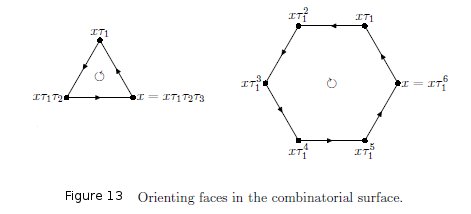
The first set in the definition of F is the set of triangular faces, while the other three are the τi faces. Assign triangular faces a positive (anticlockwise) orientation, and assign τi faces negative (clockwise) orientation. Now glue the faces together where they share a common directed edge xτi = y, ensuring that edges come together with opposite orientation.
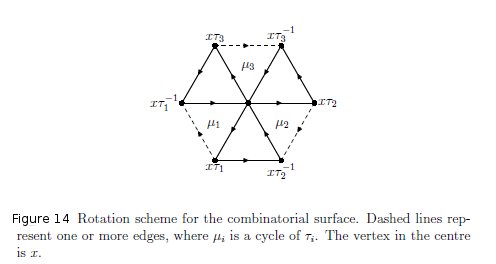
The orientation of a triangular face is shown in Figure 13 along with the orientation for a τi face. For the sake of concreteness we have illustrated a 6-cycle face due to a 6-cycle of τ1. Figure 14 shows the rotation scheme for an arbitrary vertex in the surface.
For a bitrade T = (T*, T∆) with representation [τ1; τ2; τ3] on the set Ω
, define order(T) = z(τ1) + z(τ2) + z(τ3), the total number of cycles, and
size(T) = |Ω|, the total number of points that the τi act on. By some basic counting arguments we find that there are size(T) vertices, 3 * size(T) edges,
and order(T)+size(T) faces. Then Euler's formula V - E+F = 2 - 2g gives
order(T) = size(T) + 2 - 2g
where g is the genus of the combinatorial surface. We say that the bitrade
T has genus g. A spherical bitrade has genus 0.
Example 2.2. The following bitrade is spherical:
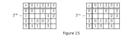
Here, the τi representation is
τ1 = (000, 022, 044)(134, 142)(201, 213, 232, 220)(304, 333, 311)
τ2 = (000, 304, 201)(213, 311)(022, 220)(134, 232, 333)(044, 142)
τ3 = (000, 220)(201, 311)(022, 232, 142)(213, 333)(044, 134, 304)
where the triples i j k refer to entries (i, j, k) ∈ T*.
We will generally assume that a bitrade is separated, that is, each row, column, and symbol is in bijection with a cycle of τ1, τ2, and τ3, respectively. We now describe how to go from a separated spherical latin bitrade to a triangle dissection (for more details see [13]). Let T = (T*, T∆) be a latin bitrade. It is natural to have different unknowns for rows, columns and symbols, and so we assume that ai ≠ bj whenever (a1, a2, a3), (b1, b2, b3) ∈ T* and 1 ≤ i < j ≤ 3. (If the condition is violated, then T can be replaced by an isotopic bitrade for which it is satisfied.) Fix a triple a = (a1, a2, a3) ∈ T* and form the set of equations Eq(T) consisting of a1 = 0, a2 = 0, a3 = 1 and b1 + b2 = b3 if (b1, b2, b3) ≠ (a1, a2, a3) and (b1, b2, b3) ∈ T*. The theorem below shows that if T is a spherical latin bitrade then Eq(T, a) always has a unique solution in the rationals. The pair (T, a) will be called a pointed bitrade.
Write ɍi, ȼj , ȿk for the solutions in Eq(T, a) for row variable ri, column variable cj, and symbol variable sk, respectively. We say that a solution to Eq(T, a) is separated if ɍi ≠ ɍï whenever i ≠ ï (and similar for columns and symbols).
For each entry c = (c1, c2, c3) ∈ T∆ we form the triangle ∆(c, a) which is bounded by the lines y = ȼ1, x = ȼ2, x + y = ȼ3. Of course, it is not clear that ∆ is really a triangle, i. e. that the three lines do not meet in a single point. If this happens, then we shall say that ∆(c, a) degenerates. Let ∆(c, a) denote the subset of T∆ such that ∆(c, a) does not degenerate. A separated dissection with m vertices corresponds to a separated spherical bitrade (T*, T∆) where |T*| = m - 2. One of the main results of [13] is the following theorem:
Theorem 2.3 ([13]). Let T = (T*, T∆) be a spherical latin bitrade, and suppose that a = (a1, a2, a3) ∈ T* is a triple such that the solution to Eq(T, a) is separated. Then the set of all triangles ∆(c, a), ∈ T∆, dissects the triangle ∑ = {(x, y); x ≥ 0, y ≥ 0 and x + y ≤ 1}. This dissection is separated.
An equilateral dissection can be obtained by applying the transformation.
(x, y) → (y/2 + x, √3y/2).Example 2.4.
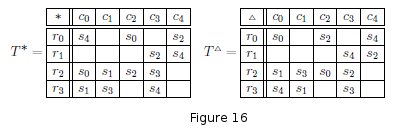
Consider the following spherical bitrade (T*, T∆):
Let a = (a1, a2, a3) = (r0, c0, s4). Then the system of equations Eq(T, a)
has the solution
ɍ0 = 0, ɍ1 = 2/7, ɍ2 = 5/14, ɍ3 = 4/7
ȼ0 = 0, ȼ1 = 3/14, ȼ2 = 5/14, ȼ3 = 3/7, ȼ4 = 5/7
ȿ0 = 5/14, ȿ1 = 4/7, ȿ2 = 5/7, ȿ3 = 11/14, ȿ4 = 1.
The dissection is shown in Figure 16. Entries of T∆ correspond to triangles
in the dissection.
For example, (r0, c0, s0) ∈ T∆ is the triangle bounded by
the lines y = ɍ0 = 0, x = ȼ0 = 0, x + y = ȿ0 = 5/14 while (r1, c3, s2) ∈ T*
corresponds to the intersection of
the lines y = ɍ1 = 2/7, x =ȿ3 = 3/7,
x + y = ȿ2 = 5/7.
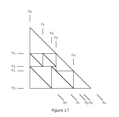
Figure 17: Separated dissection for a spherical bitrade.
The labels ri, cj , sk, refer to lines y = ɍi, x = ȼj , x + y = ȿ0, respectively.
The trade T* has 12 entries and the dissection has 12 + 2 = 14 vertices.
Applying the transformation
(x, y) → (y/2 + x, √3y/2) gives an equilateral dissection.
Dissection Results
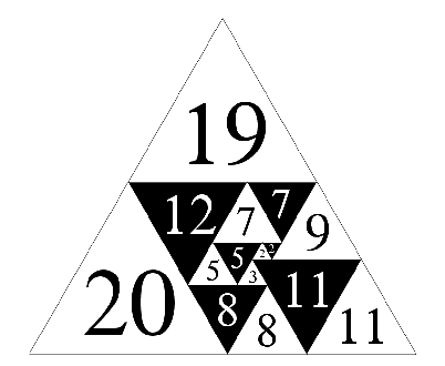
Figure 18; lowest order (15 or 7½) equilateral triangle
dissected by equilateral triangles, of size 39.
Using their enumeration code[17] Aleš Drápal and Carlo Hämäläinen confirm W. T. Tutte's conjecture [2,6] that the lowest order equilateral triangle dissection has order 15 (or 7½) and size 39 (see Figure 18). This was previously confirmed by Augusteijn in 1980 [25]. The dissections of order 16 are shown in Figures 18, and 19. The perfect dissections of orders up to 20 are available in PDF format [16] linked from the table below, and here.
In comparing the results of Augusteijn with Drápal and Hämäläinen it is worth noting Drápal and Hämäläinen double the order number of their dissections and call dissections 'perfect' which Augusteijn would separate into 'simple perfect' and 'compound perfect' (For Augusteijn, a triangulated triangle is perfect if it does not contain any sub-triangulated triangle or parallellogram). Although triangulated triangles and parallellograms always have at least two triangles the same size, if they occur only once in a dissection, and are oriented in different directions (up and down) they can be treated as different and classified as perfect. The following table summarises the known number of isomorphism classes of (numbered) Drápal and Hämäläinen perfect dissections:
| n | # perfect dissections |
|---|---|
| 15 | 2 |
| 16 | 2 |
| 17 | 6 |
| 18 | 23 |
| 19 | 64 |
| 20 | 181 |
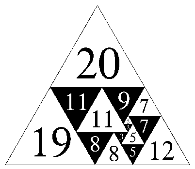
Figure 19; lowest order dissected equilateral
triangle , the 2nd of this order, an isomer of the first
The following table summarises the known number of isomorphism classes of all (unnumbered) separated (imperfect and compound) equilateral triangle dissections:
| n | #all separated dissections |
|---|---|
| 4 | 1 |
| 6 | 1 |
| 7 | 2 |
| 8 | 3 |
| 9 | 8 |
| 10 | 20 |
| 11 | 55 |
| 12 | 161 |
| 13 | 478 |
| 14 | 1496 |
| 15 | 4804 |
| 16 | 15589 |
The Padovan/Perrin Sequence and Equilateral Triangle Dissections
And now the sequence of events in no particular order. (Dan Rather)
The sequence was described by Ian Stewart in his Scientific American column Mathematical Recreations in June 1996 [21] and called the Padovan sequence. This sequence was discussed by Edouard Lucas in 1878 [20], who noted that if p is a prime then p divides s(p). This is an immediate consequence of Fermat's Little Theorem, and as such is a necessary but not sufficient condition for primality . Subsequently (1899) the same sequence was mentioned by R. Perrin [22]. The most extensive (published) treatment of this sequence was given in an excellent paper by Dan Shanks and Bill Adams in 1982 [23]. Shanks and Adams referred to this as Perrin's sequence. The Padovan sequence is named after Richard Padovan who attributed its discovery to Dutch architect Hans van der Laan in his 1994 essay Dom. Hans van der Laan : Modern Primitive [18]., to quote Richard Padovan;
"The plastic number, discovered by Dom Hans van der Laan (1904-91) in 1928 shortly after he had abandoned his architectural studies and become a novice monk, differs from all previous systems of architectural proportions in several fundamental ways. Its derivation from a cubic equation (rather than a quadratic one such as that which defines the golden section) is a response to the three-dimensionality of our world. It is truly aesthetic in the original Greek sense, i.e., its concern is not 'beauty' but clarity of perception. Its basic ratios, approximately 3:4 and 1:7, are determined by the lower and upper limits of our normal ability to perceive differences of size among three-dimensional objects. The lower limit is that at which things differ just enough to be of distinct types of size. The upper limit is that beyond which they differ too much to relate to each other; they then belong to different orders of size. According to Van der Laan, these limits are precisely definable. The mutual proportion of three-dimensional things first becomes perceptible when the largest dimension of one thing equals the sum of the two smaller dimensions of the other. This initial proportion determines in turn the limit beyond which things cease to have any perceptible mutual relation. Proportion plays a crucial role in generating architectonic space, which comes into being through the proportional relations of the solid forms that delimit it. Architectonic space might therefore be described as a proportion between proportions."[18]
The Padovan Sequence and Perrin Sequence are defined by the third-order linear recurrence relation
P(n+3) = P(n+1) + P(n). or
P(n) = P(n- 2) + P(n-3) for n>2
Both sequences satisfy the recurrence relation
P(n+5) = P(n+4) + P(n)
The two sequences differ in their initial values. In the Padovan Sequence (OEIS A000931), P(0) = 1, P(1) = 1, and P(2) = 1. The first several dozen terms of this integer sequence are;
1, 1, 1, 2, 2, 3, 4, 5, 7, 9, 12, 16, 21, 28, 37, 49, 65, 86, 114, 151, 200, 265, 351, 465, 616, 816, 1081, 1432, 1897, 2513, 3329, 4410, 5842, 7739, 10252, 13581, 17991, 23833, 31572, 41824, 55405, 73396, 97229, 128801, 170625,...
In the Perrin Sequence (OEIS A001608), P(0) = 3, P(1) = 0, and P(2) = 2 and the first several dozen terms of this sequence are;
3, 0, 2, 3, 2, 5, 5, 7, 10, 12, 17, 22, 29, 39, 51, 68, 90, 119, 158, 209, 277, 367, 486, 644, 853, 1130, 1497, 1983, 2627, 3480, 4610, 6107, 8090, 10717, 14197, 18807, 24914, 33004, 43721, 57918, 76725, 101639, 134643, 178364, 236282, 313007,...
In both sequences, the limiting ratio of consecutive terms is equal to the real root of the characteristic equation x³ - x - 1 = 0. The exact value is;
x = ∛ ½ + ⅙⋅sqrt(23/3) + ∛ ½ - ⅙⋅sqrt(23/3)
which is approximately equal to;
1.3247179572447460259609088544780973407344040569...
This number is known as the plastic constant or plastic number. Like the Fibonacci Sequence, the nth term of the Perrin and Padovan Sequences can be calculated explicitly with an exponential sum formula. For the Perrin and Padovan Sequences, the formula is;
P(n) = axn + byn + czn,
where x, y, and z are the roots of the equation t³ - t - 1 = 0 and the coefficients a, b, and c depend on the initial conditions P(0), P(1), and P(2).
Ideas are like rabbits. You get a couple and learn how to handle them, and pretty soon you have a dozen.(John Steinbeck)
Owen Elton in an article [19] Killing Fibonacci's Rabbits shows the close connection between the Fibonacci Sequence and the Padovan sequence. He writes; "One of the most famous sequences in mathematics is named after the Italian Leonardo Pisano Bigollo (Fibonacci to his mates). In his 1202 masterwork, Liber Abaci, he conducts a thought experiment about the growth of a population of rabbits.
Fibonacci's experiment set out the following rules:
A pair of rabbits takes a year to reach maturity. A mature pair produces a new pair of rabbits at the end of the year. The Fibonacci sequence is simply the year by year list of the number of pairs of rabbits produced by repeated application of this algorithm. It doesn't take too much thought to prove that this set of rules leads to a sequence where a particular term is the sum of the previous two. We can express this relationship using a difference equation:"
F(n) = F(n-1) + F(n-2) giving the Fibonacci sequence 1, 1, 2, 3, 5, 8, 13, 21, 34, 55, 89, 144,...
He has couple of concerns with Fibonacci's rules, like him we will only concern ourselves with the maths.
"...I'm more concerned that these rabbits appear to be immortal. Once they are mature, they just go on breeding for ever!"
"To add some gritty realism to the whole scenario, I decided to experiment with the idea of making the rabbits die after a certain number of years."
"We can see immediately that if rabbits die after one year then the first pair doesn't reach maturity, so the population becomes extinct. This isn't very interesting. Only slightly more exciting is the case when the rabbits die after one year of maturity." We have zero population growth, only 1 pair of rabbits alive at a time. ... "Things begin to get much more interesting if all rabbits die after 2 years of maturity."
With 2 year mortality we get a different sequence 1, 1, 2, 2, 3, 4, 5, 7, 9, 12, 16, 21, 28, 37, 49,... which we can see is the Padovan sequence.
“The human mind always makes progress, but it is a progress in spirals” ( Madame de Stael)
Another thing that has been mentioned is the geometrical representations of both sequences. It is well known that the Fibonacci sequence can be represented as a spiral of squares in the sizes of Fibonacci numbers inside a squared rectangle, often called the Golden Rectangle (after the golden ratio, the ratio that successive terms of the Fibonacci sequence approach in the limit) . Less well known is the representation of the Padovan sequence as a spiral of equilateral triangles in the sizes of the Padovan sequence. In both these representations the smallest tile is of size 1 and there are several 1s in both the square spiral and the triangle spiral, therefore neither tiling is 'perfect' in the sense of Tutte et al, Bouwkamp & Duijvestijn in that 'perfect' tilings have tiles with all tiles having different sizes.

Figure 20; Fibonacci squares and Padovan equilateral triangle spirals (Owen Elton)
We can allow an infinite number of squares in the Golden Rectangle (we can say the Rectangle is of order infinity). We can allow the rectangle to spiral outwards to infinity, or we can begin with a rectangle in the proportions of the Golden Mean, place a square at the short end and spiral inwards continuing this process recursively. If we spiral inwards then no two squares are the same size and we have a perfect Golden Rectangle of order infinity. An example was shown in Martin Gardners 1962 publication "More Mathematical Games and Puzzles'
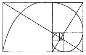
Figure 21; Golden Rectangle of Order Infinity
A Perfect Equilateral Triangle Dissection of Order Infinity.
“You have wakened not out of sleep, but into a prior dream, and that dream lies within another, and so on, to infinity, which is the number of grains of sand. The path that you are to take is endless, and you will die before you have truly awakened.” (Jorge Luis Borges)
Is it possible to perform a similar construction to the Golden Rectangle with the Padovan triangle spiral, and do it in such a way that it dissects an equilateral triangle perfectly? Indeed it is. This was done by Bernhard Klaassen in a 1995 paper; 'Infinite perfekte Dreieckszerlegungen auch für gleichseitige Dreiecke', Elem. Math. 50 (1995).. (Google translation; Infinite perfect triangular decompositions for equilateral triangles) [24]
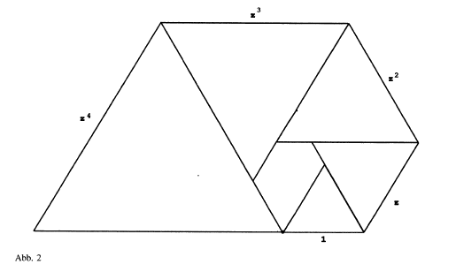
Figure 22; Padovan equilateral triangle spiral
To summarize his paper:
- First he constructs the Padovan spiral tiling. The tiling makes an irregular pentagon, with a smaller pentagon of the same shape contained within it. We can therefore spiral outwards or inwards to infinity.
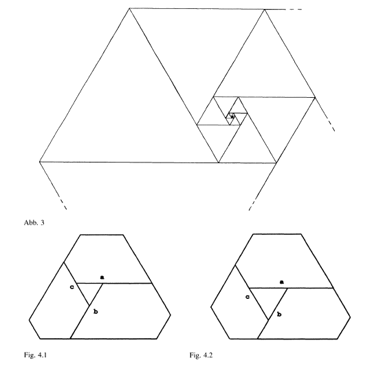
Figure 23; Padovan pentagons
- Then he takes the pentagon generated by this spiral and arranges three of them around a central triangle (one has to find the non-symmetric cases, Fig. 4.1 and 4.2)
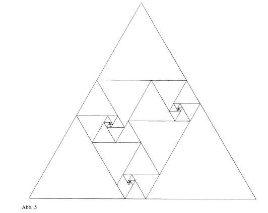
Figure 24; A Perfect Equilateral Triangle Dissection of Order Infinity
- Finally (section 3) he writes down the algebraic conditions to generate one of these cases The resulting system turns out to be linear and easy to solve, resulting in a perfect equilateral triangle dissection of order infinity.
Edited..... 14th July 2018.
References
- R.L. Brooks, C.A.B. Smith, A.H. Stone and W. T. Tutte. 'The Dissection of Rectangles into Squares'. Duke Math. J. 7 (1940) 312–340.
- W. T. Tutte, 'Dissections into Equilateral Triangles, The Mathematical Gardner, edited by David Klarner. Published by Van Nostrand Reinhold (1981)
- Aleš Drápal and Carlo Hämäläinen (July, 2010 ) :An enumeration of equilateral triangle dissections. (Discrete Applied Mathematics, Volume 158 Issue 14,)
- W. T. Tutte, Duality and Trinity. Colloquia Mathematica Societatis Janos Bolyai. 10: 1459-1472.
- R.L. Brooks, C.A.B. Smith, A.H. Stone and W. T. Tutte .1975 Leaky Electricity and Triangulated Triangles, Phillips Research Reports 30: 205-219.
- W. T. Tutte, 'The Dissection of Equilateral Triangles into Equilateral Triangles. 1948 Proc. Cambridge Phil. Soc 44: 463-482.,
- W. T. Tutte, "Graph Theory as I Have Known It". 1998, Oxford Science Publications, Clarendon Press, Chapter 4 "Unsymmetrical Electricity".
- N. J. Cavenagh and P. Lisoněk: Planar eulerian triangulations are equivalent to spherical latin bitrades, J. Combin. Theory Ser. A 15 (2008), 193–197.
- A. Drápal, Dissections of equilateral triangles and pointed spherical latin bitrades, submitted.
- J. D. Skinner, C. A. B. Smith, W. T. Tutte, On the dissection of rectangles into right-angled isosceles triangles, J. Combin. Theory Ser. B 80 (2) (2000) 277-319.
- A. Drápal, Geometrical structure and construction of latin trades, Advances in Geometry 9 (3) (2009) 311-348.
- A. Drápal, Geometry of latin trades, manuscript circulated at the conference Loops, Prague (2003).
- A. Drápal, Hamming distances of groups and quasi-groups, Discrete Math. 235 (1-3) (2001) 189-197, combinatorics (Prague, 1998).
- A. Drápal, V. Kala, C. Hämäläinen, Latin bitrades, dissections of equilateral triangles and abelian groups, Journal of Combinatorial Designs, Volume 18 Issue 1 (2010), 1-24.
- C. Hämäläinen, Latin bitrades and related structures, PhD in Mathematics, Department of Mathematics, The University of Queensland (2007)
- C. Hämäläinen, Triangle dissections code, http://bitbucket.org/ carlohamalainen/dissections.
- C. Hämäläinen, Spherical bitrade enumeration code, http:// bitbucket.org/carlohamalainen/spherical
- Richard Padovan, "Dom Hans Van Der Laan and the Plastic Number", pp. 181-193 in Nexus IV: Architecture and Mathematics, eds. Kim Williams and Jose Francisco Rodrigues, Fucecchio (Florence): Kim Williams Books, 2002.
- Owen Elton , Mathematics Teacher ,Godalming, Surrey, United Kingdom. Killing Fibonacci's Rabbits
- Edouard Lucas, 1878 (American Journal of Mathematics, vol 1, page 230ff)
- Ian Stewart, 'Tales of a Neglected Number', Scientific American column Mathematical Recreations, June 1996.
- R. Perrin (1899) (L'Intermediaire Des Mathematiciens)
- Dan Shanks and Bill Adams , (1982) (Mathematics of Computation, vol 39, n. 159)
- Bernhard Klaassen, 'Infinite perfekte Dreieckszerlegungen auch für gleichseitige Dreiecke', Elem. Math. 50 (1995).
- Lex Augusteijn, TRIANGULATIONS bachelor's thesis 1980, Technische Hogeschool Twente.