Stephen Johnson

A Random Search for Squared Squares

Stephen Johnson has kindly contributed the following article, in which describes his random search method for squared squares, which he has employed to good effect over the last couple of years.

In 2010 I began writing a program to search for squared squares. Rather than exhaustively check all graphs of a certain size, the method is a random (but crudely directed) search for squared rectangles, trying to drive the aspect ratio (height/width) to unity. My method for finding squared squares is a random search, somewhat guided by a few simple heuristic rules. The basic idea is to begin with any rectangular dissection, then modify its analogous electrical network description in order to change the rectangle proportions to make it more like a square (either taller or wider). If it doesn't become exactly square, continue by modifying the new dissection. I call the computer program "crawl" because A) it is slow; and B) I think of it as crawling back and forth across the range of possible height/width ratios, trying to find rectangles with ratio exactly 1.0.

It begins with a randomly generated rectangular dissection, somewhere in the range of order 25 to 30. The rectangle may be "tall" or "wide", perfect or imperfect, but it must not be compound. The dissection is described simultaneously in 3 different ways: as an ordered set of squares; as a list of "electrical network" node pairs; and as a list of polygons. The polygon list basically is the set of polygons which collectively form the "electrical network" description of the dissection. In 2011-2013, using this method I contributed a small fraction of the large collection of squared squares assembled at Stuart Anderson’s great web site, squaring.net.

I. The random search method

1) Begin with any squared rectangle (“dissection”).

2) Determine the graph describing the “electrical network” analogy for the dissection.

3) Decide whether we want to add or remove squares from the dissection, and whether we want to make it wider or taller (to become more square).

4) Based on the assessment in #2, pick one of four different methods, of altering the graph. These involve splitting a node into two, merging two nodes, etc. More details on the alteration methods are given below.

5) For the altered graph, determine the new rectangle dissection, and the new height and width. If it is a squared square, print it out.

6) Replace the previous graph with the new one, and go back to step 2. Continue for many thousands of iterations.

After several “tweaks” applied to help the process run smoothly, the program now cycles through steps 2 through 6 millions of times in a day, crossing back and forth across the unity line (height equals width) about once every 4 alterations, cycling the order (number of component squares) between 29 and 36, and finding a handful of squared squares in the process.

II. Methods of altering the graph

Here are examples of each of the four methods for altering the graph, with before-and-after illustrations of the dissection and its corresponding graph.

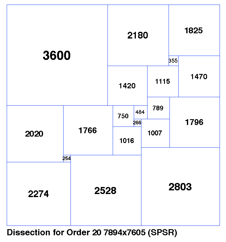
Suppose our current dissection is the Order-20 graph shown in Figure 1. This rectangle’s height exceeds its width, so we want to make it wider. Also we are targeting squared squares in the range of orders 29-36, so we want to add a square. The method for that is “split polygon”.

Figure 1: Order 20 dissection, 7894 X 7605

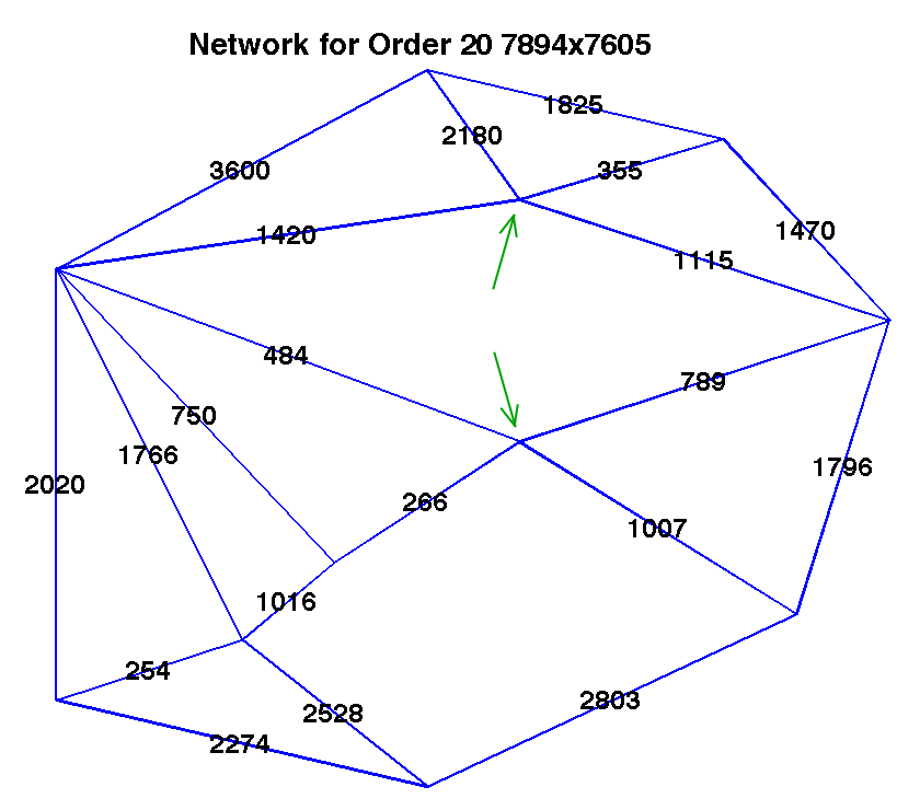
In Figure 2, we have the graph (network) representing this dissection. The graph edges are labeled, showing the sizes of the corresponding squares. The graph includes two polygons with 4 or more vertices each. We randomly pick one of those 2 polygons, and then (within that polygon) we randomly pick a pair of non-adjacent vertices. These two vertices are indicated by 2 green arrows.

Figure 2: Order 20 graph

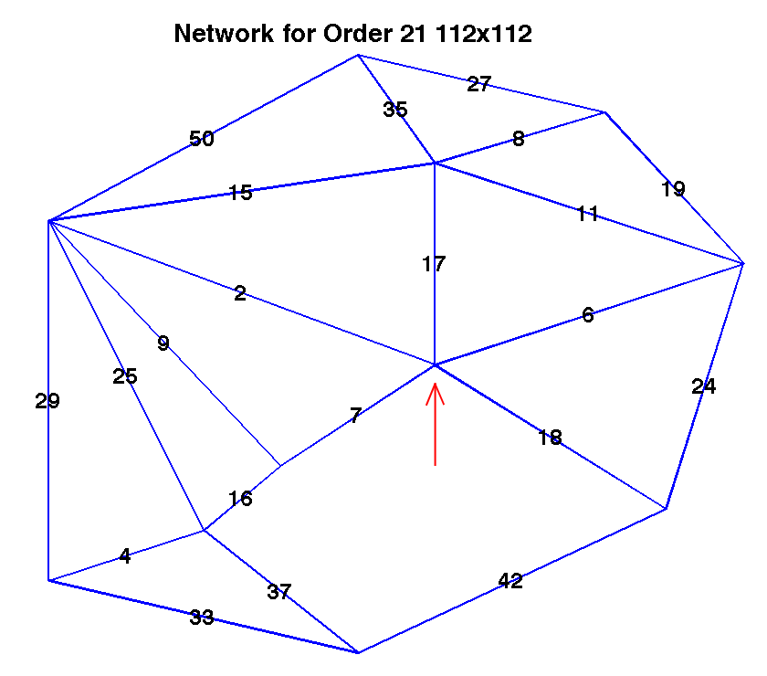
Having made that connection, we then convert from the new graph, to a dissected rectangle with one more square (Order 21). The results are shown in Figures 3 and 4. The new edge (connection) we have made has length 17 in the new “solved” network in Figure 4.

Figure 3: Order 21 dissection, 112 X 112

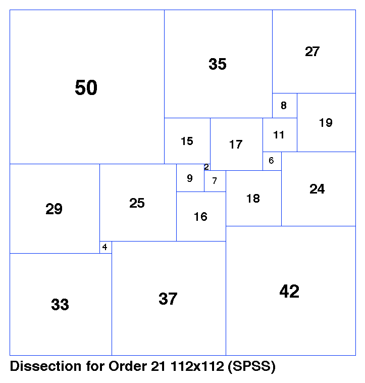
Figure 4: Order 21 graph

Since this is a squared square, we print out the dissection, and continue.

Suppose we decide to increase the order again, but this time drive the rectangle to be taller, not wider. The method for that is “split node”. In Figure 4, this can be applied in multiple places. There are 5 different nodes with at least 4 connections each; and each such node can be split in multiple ways. We will randomly choose the node indicated by a red arrow, keeping the top three edges with one “child node”, and remaining (bottom two) edges with the other “child node”.

The resulting graph is in Figure 6, and the corresponding dissected rectangle is in Figure 5. The two “child nodes” from the split are connected by a new edge (square, in the dissection) shown with length 8400. One more node means one more square, so this is Order 22.

Figure 5: Order 22 dissection, 70274 X 68399

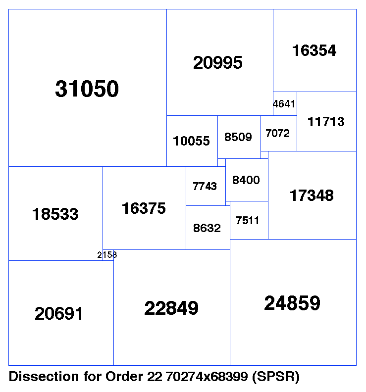
Figure 6: Order 22 graph

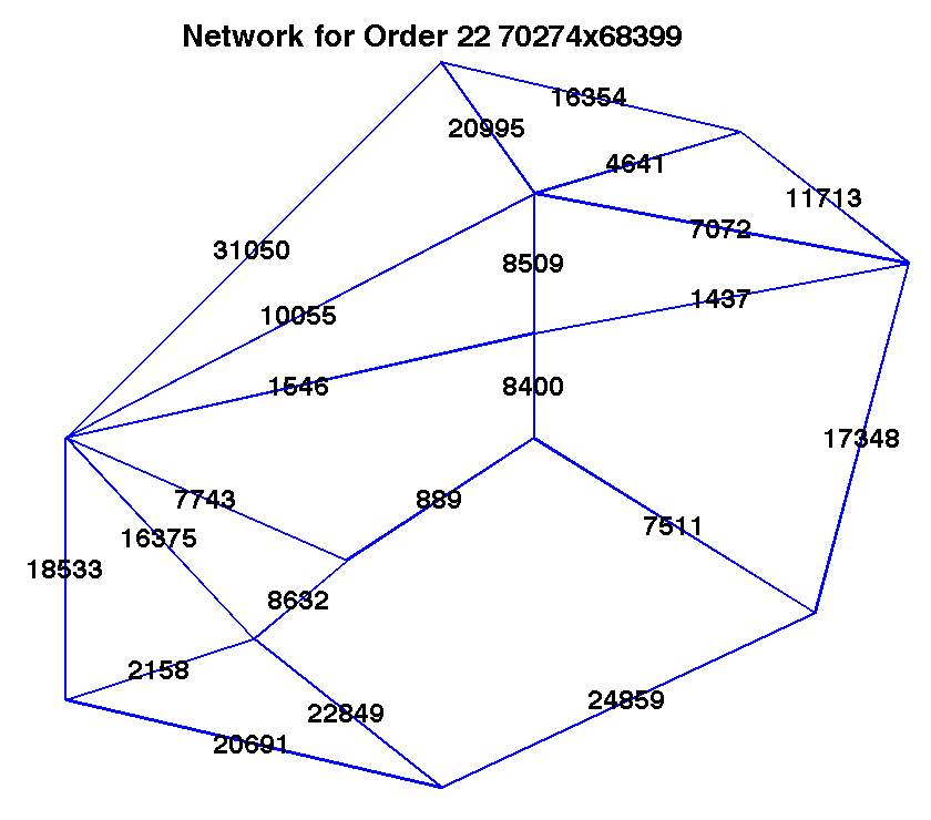
To reduce the order (remove a square), we can make the rectangle wider using “merge nodes”, which is the reverse of the process between Figures 4 & 6. To reduce order and make it taller, we “remove edge”, which reverses the process from Figure 2 to Figure 4.

In summary our 4 options are:

	Increase Order	Decrease Order
Make wider	Split Polygon	Merge Nodes
Make taller	Split Node	Remove Edge

Other methods can be used to alter a graph. Two others I call “pinch poly” (not currently active in my program) and “pivot edge” (see below).

III. Code details

A) In order to avoid getting stuck in an endless loop, several additional alterations/interruptions are included at infrequent intervals during the search. These include “pivot edge”, a different way to modify the graph; “rotate 90”, which means rotate the rectangle so that its two “sides” become the new top and bottom (the “poles” for the graph); and start over, i.e. throw out the current dissection and generate a new random one as in step 1.

B) The two choices at step 3 (whether to add or remove squares, and whether to drive the rectangle taller or wider) include a small random factor, again to avoid getting stuck.

C) In order to avoid many complications, whenever the program encounters a zero-length square, or two “side by side” identical squares, or a compound dissection, it rejects that dissection and tries something else. Ideally a “smarter” program would be able to deal with these cases, but I found it easier to simply back up and go in a different direction.

D) Steps 2 and 5 involve converting back and forth, between the graph (nodes and connecting edges) description, and the rectangular dissection (square sizes and locations). To repeatedly perform these conversions (reasonably quickly) required writing many functions and maintaining several different, simultaneous, parallel descriptions of the current dissection. These are a “connection matrix”; a list of the perimeter nodes in the graph; a list of connective edges in the graph; a list of the smallest polygons which together form the graph; the tablecode (Bouwkamp description); etc.

E) The C program is called “crawl.c” because it crawls back and forth over the unity boundary (rectangle height/width).

The code has been posted to the downloads page of this site.