Brooks, Smith, Stone, Tutte (Part II)
A number of accounts have related how Arthur Stone was the first of the four undergraduates to raise the problem of the squared square. CAB Smith in personal communication to Skinner states;
"W.R. Dean is largely responsible for the development of the idea of squaring the square - he visited Arthur Stone's school before Arthur came to Cambridge and said that an unsolved problem was to show that a square can not be dissected into a finite number of unequal squares. He later became Professor of Applied Mathematics at University College, London."
We know that this time was at or prior to 1935. The extant publications were few (the Dehn paper (1903), Loyd's(1914) and Dudeney's(1902, 1907-19) Puzzles, the Moron' paper(1925), the Abe papers (1930,31) and the Kraitchik paper(1930). Kraitchik published a personal communication from Russian mathematician N.N. Lusin which stated that it was impossible to dissect a square into a finite number of different elements. This became known as Lusin's conjecture.
The paper they co-authored at the conclusion of their investigation, "The Dissection of Rectangles into Squares;" Ranged across a variety of mathematical disciplines; Electrical network theory, planar graphs, 3-connection, duality, the matrix-tree theorem, number theory, and determinants.
The main results were;
- Every squared rectangle has commensurable sides and elements.
- Every rectangle with commensurable sides is perfectible in an infinity of different ways.
- Discovery of spss order 39 (not shown), and cpss order 26 (empirical).
- No perfect rectangles order less than 9. There are 2 perfect rectangles of order 9.
- Generalisations of the problem; rectangled rectangles, squared cylinders and tori, triangled equilateral triangles and a proof of no cubed cubes.
The story of how the four Cambridge undergraduates solved the problem has been told by various authors. In my view the best account is given by W.T. Tutte himself in the article he wrote for Martin Gardners book 'More Mathematical Puzzles and Diversions'[1].
Squaring the Square,
W. T. Tutte
William Thomas Tutte
This is the story of a mathematical research conducted by four students of Trinity College, Cambridge, in the years 1936-8. One was the author of this article. Another was Cedric Smith, now a statistical geneticist at the University of London. He is also well known as a writer on the theory of games and the counterfeit-coin problem. Another was A. H. Stone, now researching at Manchester into recondite regions of point set topology. He is one of the inventors of the flexagons described in Mathematical Puzzles and Diversions. The fourth was R.L. Brooks. He has now left the academic world for the Civil Service. But he retains an enthusiasm for mathematical recreations, and an important theorem in the theory of graph colourings bears his name. These four students referred to themselves, with characteristic modesty, as the 'Important Members' of the Trinity Mathematical Society.
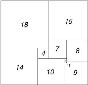
Figure 70; 33x32 Squared Rectangle
In 1936 there were a few references in the literature to the problem of cutting up a rectangle into unequal squares. Thus it was known that a rectangle of sides 32 and 33 can be dissected into nine squares with sides of 1,4,7,8,9,10,14,15, and 18 units (Figure 70). Stone was intrigued by a statement in Dudeney's Canterbury Puzzles which seemed to imply that is is impossible to cut up a square into unequal smaller squares. He tried to prove the impossibility for himself, but without success. He did, however, discover a dissection of the rectangle of sides 176 and 177 into 11 unequal squares (Figure 72).
This partial success fired the imaginations of Stone and his three friends and soon they were spending much time constructing, and arguing about, dissections of rectangles into squares. Any rectangle cut up into unequal squares was called by them a 'perfect' rectangle. Years later the term 'squared rectangle' was introduced to describe any rectangle cut up into two or more squares, not necessarily unequal.
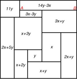
Figure 71; Algebraic Method
The construction of perfect rectangles proved to be quite easy. The method used was as follows. First we sketch a rectangle cut up into rectangles, as in Figure 71. We then think of the diagram a bad drawing of a squared rectangle, the small rectangles being really squares, and we work out by elementary algebra what the relative sizes of the squares must be on this assumption. Thus in Figure 71 we have denoted the sides of two adjacent small squares by x and y and then that the side of the square next on the left is x+2y, and so on. Proceeding in this way we get the formulae shown in Figure 71 for the sides of the 11 small squares. These formulae make the squares fit together exactly except along one segment AB. But we can make them fit on AB too by choosing x and y to satisfy the equation (3x + y) + (3x - 3y) = (14y - 3x), that is 16y = 9x . Accordingly we put x = 16 and y = 9 . This gives the perfect rectangle of Figure 72, which is the one first found by Stone.
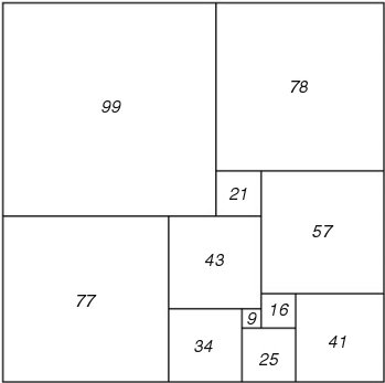
Figure 72; 177 x 176 Squared Rectangle
Sometimes this method gave negative values for the sides of some small squares. It was found, however, that such negative squares could always be converted into positive ones by minor modifications of the original diagram. They therefore gave no trouble. In some of the more complicated diagrams it proved necessary to start with three unknown squares, with sides x, y and z, and solve two linear equations instead of one at the end of the algebraic computations. Sometimes the squared rectangle finally obtained proved not to be perfect, and the attempt was considered a failure. Fortunately this did not happen very often. We recorded only 'simple' perfect rectangles, that is perfect rectangles containing no smaller ones. For example, the perfect rectangle obtained from Figure 70 by erecting a new component square of side 32 on the upper horizontal side is not simple, and we did not include it in our catalogue.
In this first stage of the research, large numbers of perfect rectangles were constructed in which the number of component squares ranged from 9 to 26. In the final form of each rectangle the sides the sides of the component squares were represented as integers without a common factor. Of course we all hoped that if we constructed enough perfect rectangles by this method we would eventually obtain one which was a 'perfect square'. But as the list of perfect rectangles lengthened this hope faded. Production slowed down accordingly.
Inspection of the catalogue we had constructed revealed some very odd phenomena. We had classified our rectangles according to their 'order', that is, the number of component squares. We noticed a tendency for numbers representing sides to be repeated in any one order. Moreover the semi-perimeter of a rectangle in one order often reappeared several times as a side in the next order. For example, using the information now available, one finds that four of the six simple perfect rectangles of order 10 have semi-perimeter 209, and that five of the 22 simple perfect rectangles of order 11 have 209 as a side. There was much discussion of this "Law of Unaccountable Recurrence", but it led to no satisfactory explanation.
In the next stage of the research we abandoned experiment in favour of theory. We tried to represent squared rectangles by diagrams of different kinds. The last of these diagrams, introduced by Smith, was a really big step forward. The other three researchers called it the Smith diagram. But Smith objected to this name arguing that his diagram was only a minor modification of one of the earlier ones. However that may be, Smith's diagram suddenly made our problem part of the theory of electrical networks.
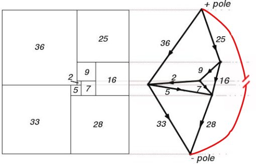
Figure 73; 69 x 61 Squared Rectangle and Smith Diagram
Figure 73 shows a perfect rectangle together with its Smith diagram. Each horizontal line-segment in the drawing is represented in the Smith diagram by a dot, or 'terminal'. In the Smith diagram the terminal is made to lie on a continuation to the right of its corresponding horizontal segment in the rectangle. Any component square of the rectangle is bounded above and below by two of the horizontal segments. Accordingly it is represented by a line or 'wire' in the diagram joining the two corresponding terminals. We imagine an electric current flowing in each wire. The magnitude of the current is numerically equal to the side of the corresponding square, and its direction is from the terminal representing the lower one.
The terminals corresponding to the upper and lower horizontal sides of the rectangle may conveniently be called the positive and negative poles, respectively, of the electrical network.
Surprisingly enough the electric currents assigned by the above rule really do obey Kirchhoff's Laws for the flow of current in a network, provided that we take each wire to be of unit resistance. Kirchhoff's First Law states that, except at a pole, the algebraic sum of the currents flowing to any terminal is zero. This corresponds to the fact that the sum of the sides of the squares bounded below by a given horizontal segment is equal to the sum of the squares bounded above by the same segment, provided of course that the segment is not one of the horizontal sides of the rectangle. The second law says that the algebraic sum of the currents in any circuit is zero. This is equivalent to saying that when we describe the circuit the net corresponding change in level must be zero.
The total current entering the network at the positive pole, or leaving it at the negative pole is evidently equal to the horizontal side of the rectangle, and the potential difference between the two poles is equal to the vertical side.
The discovery of this electrical analogy was important to us because it linked our problem with an established theory. We could now borrow from the theory of electrical networks and obtain formulae for the currents in a general Smith diagram and the sizes of the corresponding component squares. The main results of this borrowing can be summarized as follows. With each electrical network there is a number calculated from the structure of the network, without any reference to which particular pair of terminals is chosen as poles. We called this number the complexity of the network. If the units of measurement for the corresponding rectangle are chosen so that the horizontal side is equal to the complexity, then the sides of the component squares are all integers. Moreover, the vertical side is equal to the complexity of another network obtained from the first by identifying the two poles.
The numbers giving the side of the rectangle and its component squares in this system of measurement were called the full sides and full elements of the rectangle respectively. For some rectangles the full elements have common factor greater than unity. In any case division by their common factor gives the 'reduced' sides and elements. It was the reduced sides and elements that had been recorded in our catalogue.
These results imply that if two squared rectangles correspond to networks of the same structure, differing only in the choice of poles, then the full horizontal sides are equal. Further if two rectangles have networks which acquire the same structure when the two poles of each are identified, then the full horizontal sides are equal. Further, if two rectangles have networks which acquire the same structure when the poles of each are identified, then the two vertical sides are equal. These two facts explained all the cases of 'unaccountable recurrence' which we had encountered.
The discovery of the Smith diagram simplified the procedure for producing and classifying simple squared rectangles. It was an easy matter to list all the permissible electrical networks of up to 11 wires and to calculate all the squared rectangles. We then found that there were no perfect rectangles below the 9th order, and only 2 of the ninth(Figures 70 and 73). There were six of the 10th order and 22 of the 11th. The catalogue then advanced, though more slowly, through the 12th order (67 simple perfect rectangles) and into the 13th.
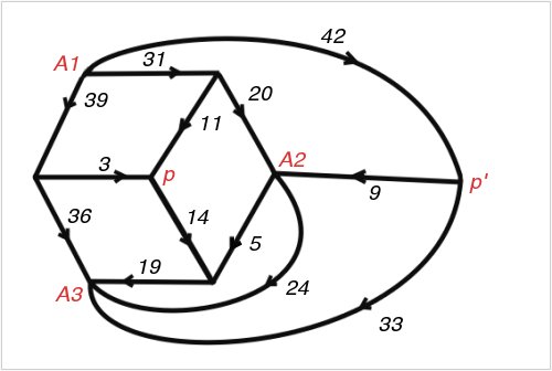
Figure 74; 112 x 75A Smith Diagram
It was a pleasing recreation to work out perfect rectangles corresponding to networks with a high degree of symmetry. We considered, for example, the network defined by a cube, with corners for terminals and edges for wires. This failed to give any perfect rectangles. However, when complicated by a diagonal wire across one face, and flattened into a plane, it gave the Smith diagram of Figure 74 and the corresponding squared rectangle of Figure 75. This rectangle is especially interesting because its reduced elements are unusually small for the thirteenth order. The common factor of the elements is six. Brooks was so pleased with this rectangle that he made a jigsaw puzzle of it, each of the pieces being one of the component squares.
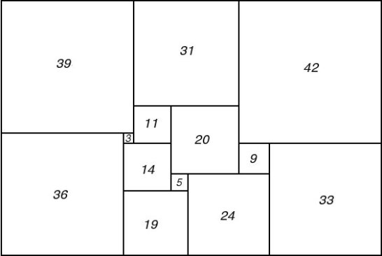
Figure 75; 112 x 75A Squared Rectangle
It was at this stage that Brooks's mother made the key discovery of the whole research. She tackled Brooks's puzzle and eventually succeeded in putting the pieces together to form a rectangle. But it was not the squared rectangle which Brooks had cut up!
Brooks returned to Cambridge to report the existence of two different perfect rectangles with the same reduced sides and the same reduced elements. Here was unaccountable recurrence with a vengeance! the Important Members met in emergency session.
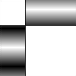
Figure 76; Perfect Square, Two Rectangles
We had sometimes wondered whether it was possible for different perfect rectangles to have the same shape. We would have liked to obtain two such rectangles with no common reduced element, and thus get a perfect square by the construction shown in Figure 76. The shaded regions in this diagram represent the two perfect rectangles. Two unequal squares were then added to make the large perfect square. But no rectangles of the same shape had hitherto appeared in our catalogue, and we had reluctantly come to believe that the phenomenon was impossible. Mrs Brooks's discovery renewed our hopes, even though her rectangles failed in the worst possible way to have no common reduced element.
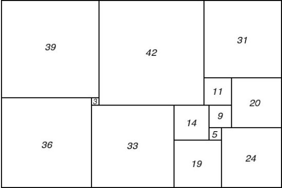
Figure 77; 112 x 75B Squared Rectangle
There was much excited discussion at the emergency session. Eventually the Important Members calmed down sufficiently to draw the Smith diagrams of the two rectangles. Inspection of these soon made clear the relationship between them.
The second rectangle is shown in Figure 77 and its Smith diagram in Figure 78. It is evident that the network of Figure 78 can be obtained from that of Figure 74 by identifying the terminals p and p'. As p and p' happen to have the same electrical potential in figure 74 this operation causes no change in the currents in the individual wires, no change in the total current, and no change in the potential difference between the poles. We thus have a simple electrical explanation of the fact that the two rectangles have the same reduced sides and the same reduced elements.
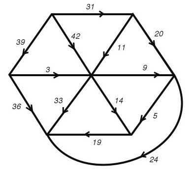
Figure 78; 112 x 75B Smith Diagram
But why do p and p' have the same potential in figure 74? Before the emergency session broke up it had obtained an answer to this question also. The explanation depends on the fact that the network can be decomposed into three parts meeting only at the poles A1 and A2 and the terminal A3. One of these parts consists solely of the wire joining A2 and A3. A second part is made up of the three wires meeting at p', and a third is constituted by the remaining nine wires. Now the third part has threefold rotational symmetry with p as the centre of rotation. Moreover, current enters or leaves this part of the network only at A1, A2 and A3, which are equivalent under the symmetry. This is enough to ensure that if any potentials whatever are applied to A1, A2, and A3 the potential of p will be their average. The same argument applied to the second part of the network shows that the potential of p' must also be the average of the potentials A1, A2 and A3. Hence p and p' have the same potential, whatever potentials are applied to A1, A2 and A3, and in particular they have the same potential when A1 and A2 are taken as poles in the complete network, and the potential of A3 is fixed by Kirchhoffs Laws.
The next advance was made accidently by the present writer. We had just seen Mrs Brook's discovery completely explained in terms of a simple property of symmetrical networks. It seemed to me that it should be possible to use this property to construct other examples of pairs of perfect rectangles with the same reduced elements. I could not have explained how this would help us in our main object of of constructing, or proving the impossibility of, a perfect square. But I thought we should explore the possibilites of the new idea before abandoning them.
The obvious thing to do was to replace the third part of the network of Figure 74 by another network having threefold rotational symmetry about a central terminal. But this can be done only under severe limitation, which should now be explained.
It can be shown that the Smith diagram of a squared rectangle is always planar, that is, it can be drawn in the plane with no crossing wires. And the drawing can always be made so that no circuit separates the two poles. There is also a converse theorem which states that if an electrical network of unit resistances can be drawn in the plane in this way, then it is the Smith diagram of some squared rectangle. It would not be proper to take up space in this book with rigorous proofs of these theorems. It would not even be historically accurate; the four researchers did without rigorous proofs right up to the time when they began to prepare their technical paper for publication.
It is not always advisable to disregard rigour in this way in the course of a mathematical research. In research aiming at a proof of the Four Colour Theorem, for example, such an attitude would be, and often is, disastrous. But our research was largely experimental, and its experimental results were perfect rectangles. Our methods were justified, for the time being, by the rectangles they produced, even when their theory had not been precisely worked out.
But let us return to Figure 74 and the replacement of its third part by a new symmetrical network with centre p. The complete network obtained in this way must not only be planar but it must remain planar when p and p' are identified.
After a few trials I found two closely related networks satisfying these conditions. The corresponding Smith diagrams are shown in figures 79 and 80. As expected, each diagram allowed of the identification of p and p', and so gave rise to two squared rectangles with the same reduced elements. But all four rectangles had the same reduced sides, and this result was unexpected.
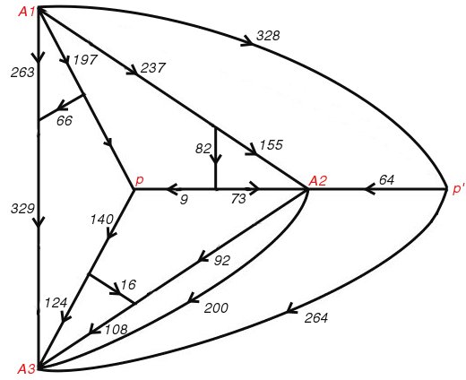
Figure 79; Smith Diagram
Essentially the new discovery was that the rectangles corresponding to Figures 79 and 80 have the same shape, though they do not have their reduced elements all the same. A simple theoretical explanation of this was soon found. The two networks have the same structure, apart from the choice of poles, and therefore the rectangles have the same full horizontal side. Moreover the networks remain identical when poles are coalesced, and therefore the two rectangles have the same vertical side. We felt, however, that this explanation did not probe sufficiently deep, since it made no reference to rotational symmetry.
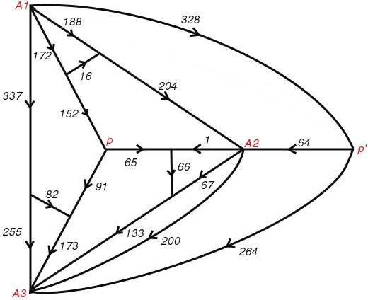
Figure 80; Smith Diagram
We eventually agreed to refer to the new phenomenon as 'rotor-stator' equivalence. It was always associated with a network which could be decomposed into two parts, the 'rotor' and the 'stator', with the following properties. The rotor had rotational symmetry, the terminals common to the rotor and stator were all equivalent under the symmetry of the rotor, and the poles were terminals of the stator. In Figure 79, for example, the stator is made up of the three wires joining p' to A1, A2, and A3, and the wire linking A2 with A3. A second network could then be obtained by an operation called 'reversing' the rotor. With a properly drawn figure this could be explained as a reflection of the rotor in the line pA3 and so obtain the network of Figure 80.
After studying a few examples of rotor-stator equivalence the researchers convinced themselves that reversing the rotor made no difference to the currents in the wire of the stator. But the currents in the rotor might change. Satisfactory proofs of these results were obtained only at a much later stage.
Rotor-stator equivalence proved to have no very close relationship with the phenomenon discovered by Mrs Brooks. It was merely another one associated with networks having a part with rotational symmetry. The importance to us of Mrs Brooks's discovery was that it led us to study such networks.
Figure 81; Perfect Square, Shared Corner
A very tantalizing question now arose. What was the least possible number of common elements in a rotor-stator pair of perfect rectangles? Those of Figures 79 and 80 had seven common elements, three of which corresponded to currents in the rotor. The same rotor with a stator consisting of a single wire A2A3 gave two perfect rectangles of the 16th order with four common elements. Using a one-wire stator there seemed no theoretical reason why we should not obtain a pair of perfect rectangles having only one element, corresponding to the stator, in common. But we saw that if we could do this we could also obtain a perfect square. For with the rotors of threefold symmetry which we were studying, a one wire stator always represented a corner element of each corresponding rectangle. From the two perfect rectangles with only a corner element in common we can expect to obtain a perfect square by the construction illustrated in Figure 81. Here the shaded regions represent the two rectangles. The square in which they overlap is the common corner element.
Naturally we got to work calculating rotor-stator pairs. We made the rotors as simple as we could, partly to save labour and partly in the hope of getting a perfect square with small reduced elements. But one construction after another failed, because of common elements in the rotor, and we became discouraged. Was there some theoretical barrier yet still to be explored?
It occurred to some of us that perhaps our rotors were too simple. Something more complicated might be better. the numbers involved would be bigger and the likelihood of a chance coincidence would be reduced. So it came to pass that Smith and Stone sat down to compute a complicated rotor-stator pair while Brooks, unknown to them worked on another in a different part of the College. After some hours Smith and Stone burst into Brooks's room crying 'We have a perfect square!' To which Brooks replied 'So have I!'
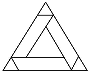
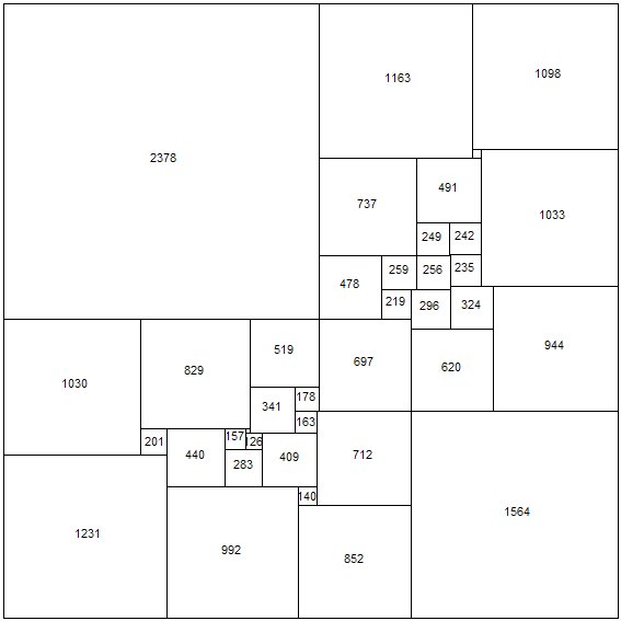
Figure 82; Brooks Perfect Square Rotor
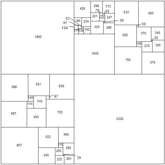
Both these squares were of the 69th order. But Brooks went on to experiment with simpler rotors and obtained a perfect square of the 39th order. This corresponds to the rotor shown in Figure 82. A brief description of it is provided by the following formula:
(2378,1163,1098) (65,1033) (737,491) (249,242) (7,235) (478,259) (256) (324,944) (219,296) (1030,829,519,697) (620) (341,178) (163,712,1564) (201,440,157,31) (126,409) (283) (1231) (992,140) (852)
In this formula each pair of brackets represents one of the horizontal segments in the subdivision pattern of the perfect square. These segments are taken in vertical order, beginning with the upper horizontal side of the square, and the lower horizontal side is omitted. the numbers enclosed by a pair of brackets are the sides of those component squares which have their upper horizontal sides in the corresponding segment. They are taken in order from left to right. The reduced side of the perfect square is the sum of the numbers in the first pair of brackets, that is 4,639.
The notation we have just used is that of C.J. Bouwkamp. He has employed it in his published list of the simple squared rectangles up to the 13th order.
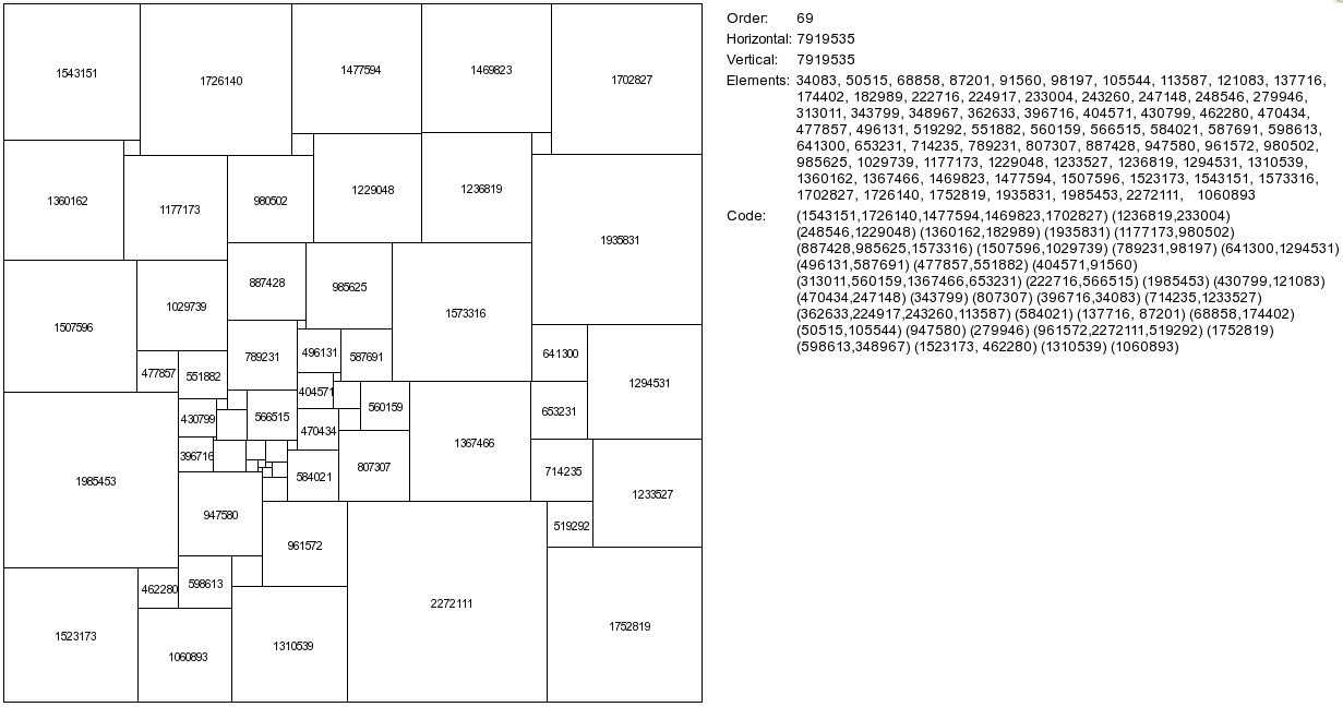
This really completes the story of how this particular team solved the problem of the perfect square. We did more work on the problem, it is true. All the perfect squares obtained by the rotor-stator method had certain properties which we regarded as blemishes. Each contained a smaller perfect rectangle; that is, was not simple. Each had a point at which four of the component squares met; that is, was 'crossed'. Finally, each had a component square, not one of the four corner squares, which was bisected by a diagonal of the complete figure. Using a more advanced theory of rotors we were able to get perfect squares without the first two blemishes. Years later, by a method based on a completely different kind of symmetry, I obtained a perfect square of the 69th order free of all three kinds of blemish. But for an account of this work I must refer the interested reader to our technical papers. [references 2.]
There are three more episodes in the history of the perfect square which ought to be mentioned, though each one may seem like an anti-climax.
To begin with, we kept adding to the list of simple perfect rectangles of the 13th order. Then one day we found that two of these rectangles had the same shape and no common element. They gave rise to a perfect square of the 28th order by the construction of Figure 76. Later we found a 13th order perfect rectangle which could be combined with one of the 12th order and one extra component square to give a perfect square of the 26th order. If the merit of a perfect square is measured by the smallness of its order, then the empirical method of cataloguing the perfect rectangles had proved superior to our beautiful theoretical method.
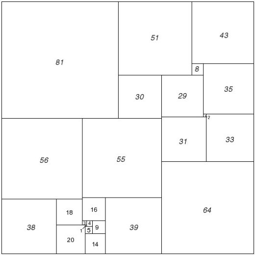
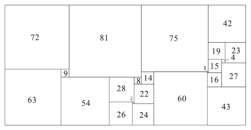
Figure 83; Willcocks 175 Compound Perfect Square
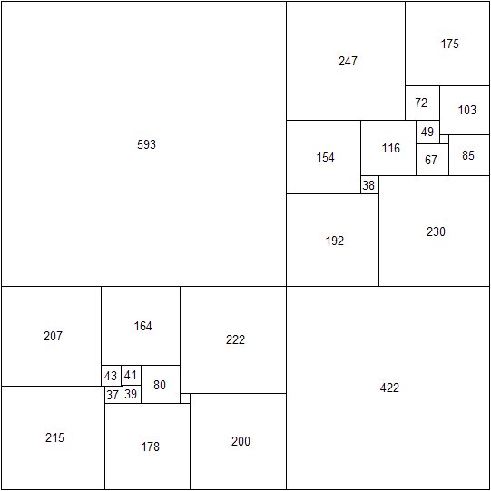
Other researchers have used the empirical method with spectacular results. R. Sprague of Berlin fitted a number of perfect rectangles together in a most ingenious way to produce a perfect square of the 55th order. This was the first perfect square to be published (1939). More recently T.H. Willcocks of Bristol, who did not confine his catalogue to simple and perfect squared rectangles, obtained a perfect square of the 24th order (Figure 83). Its formula is as follows: (55,39,81) (16,9,14) (4,5) (3,1) (20) (56,1) (38) (30,51) (64,31,29) (8,43) (2,35) (33). This perfect square still holds the low-order record. [Perfect Compound Square record, see footnote 1.]
Unlike the theoretical method, the empirical one has not yet given rise to any simple perfect square.
In case any reader should like to do some work on perfect rectangles himself, here are two unsolved problems. The first is to determine the smallest possible order for a perfect square [solved, see footnote 2.]. The second is to find a simple perfect rectangle whose horizontal side is twice the vertical side. [solved, see footnote 3.]
W.T.TUTTE
REFERENCES
- "More Mathematical Puzzles and Diversions", 1961, collection by Martin Gardner. Ch 17. 'Squaring the Square' by William T. Tutte , from 'Mathematical Games' column Nov 1958, Scientific American.
- 'Beispiel Einer Zerlegung des Quadrats in Lauter Verschiendene Quadrate' by R. Sprague in Mathematische Zeitschrift, Vol. 45, pages 607-8, 1939.
- 'A Class of Self-Dual maps' by C.A.B. Smith and W.T.Tutte in Canadian Journal of Mathematics, Vol. 2, pages 179-96, 1950.
- 'On the Construction of Simple Perfect Squared Squares' by C.J. Bouwkamp in Koninklinjke Nederlandsche Akademie van Wetenschappen, Proceedings, Vol. 50, pages 1296-99, 1947.
- 'The Dissection of Rectangles into Squares' by R.L. Brooks, C.A.B. Smith, A.H. Stone, and W.T. Tutte in Duke Mathematical Journal, vol. 7, pages 312-40, 1940.
- 'On the Dissection of Rectangles into Squares (I-III)' by C.J. Bouwkamp in Koninklinjke Nederlandsche Akademie van Wetenschappen, Proceedings, Vol. 49, pages 1176-88, 1946, and Vol. 50, pages 58-78, 1947.
- 'A Note on Some Perfect Squared Squares' by T.H. Willcocks in Canadian Journal of Mathematics, Vol. 3, pages 304-8, 1951.
- 'Question E401 and Solution' by A.H. Stone in American Mathematical Monthly, Vol. 47, pages 570-2, 1940.
- 'A Simple Perfect Square' by R.L. Brooks, C.A.B. Smith, A.H. Stone, and W.T. Tutte in Koninklinjke Nederlandsche Akademie van Wetenschappen, Proceedings, vol 50, pages 1300-1, 1947.
- 'Squaring the Square' by W.T. Tutte in Canadian Journal of Mathematics, Vol 2, pages 197-209, 1950.
- Catalog of Simple Squared Rectangles of Orders Nine Through Fourteen and their Elements by C.J. Bouwkamp, A.J.W. Duijvestijn, and P. Medema. Department of Mathematics, Technische Hogeschool, Eindhoven, Netherlands, 1960.
- 'The Dissection of Equilateral Triangles into Equilateral Triangles' by W.T.Tutte in Proceedings of the Cambridge Philosophical Society, Vol. 44, pages 464-82, 1948.
WEBMASTER FOOTNOTES
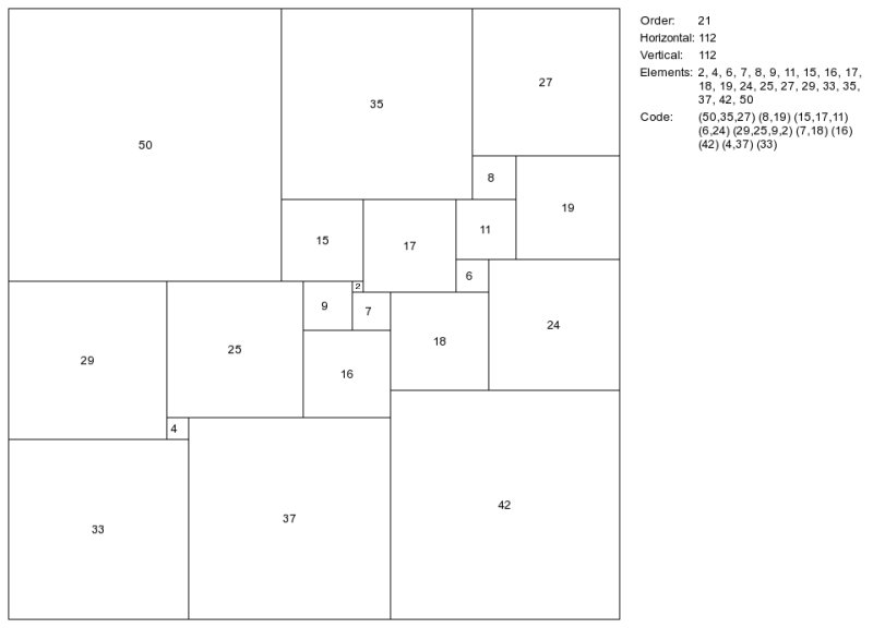
- The low order record for a perfect square is AJW Duijvesijn's order 21 square, but this order 24 square of Willcocks (Figure 83) is the lowest possible order for a compound perfect square. See 'Compound Perfect Squares' by A. J. W. Duijvestijn, P. J. Federico, P. Leeuw in The American Mathematical Monthly, Vol. 89, No. 1 (Jan., 1982), pp. 15-32
- Order 21 simple perfect squared square, found in March 1978 by AJW Duijvestijn, published 'Simple perfect squared square of lowest order', J. Combin. Theory Ser. B 25 (1978), no. 2, 240-243.
-
Brooks, R. L. "A procedure for dissecting a rectangle into squares, and an example for the rectangle whose sides are in the ratio 2:1", J. Combinatorial Theory, 10 (1971) 206-211
Order 23 2x1 simple perfect squared rectangle, discovered by P. J. Federico. Exercise 35, Ch 5, 'Tiling', 'Mathematics, The Man-Made Universe', Sherman Stein, 3rd ed., p 96.
Order 22 2x1 simple perfect squared rectangle of lowest order, found in August 1978 by AJW Duijvestijn, published 'A lowest order simple perfect 2x1 squared rectangle', J. Combin. Theory Ser. B 26 (1979), no. 3, 372-374.